

 Share This Page
| Home | | Ham Radio | | | | Share This Page |
A powerful Python-based software-defined radio (SDR)
— All content Copyright © 2020, P. Lutus — Message Page —
Latest PLSDR Version: date
Most recent update to this page:

Figure 1: PLSDR in operation
(double-click any word to see its definition)
This page describes and provides a particular software-defined radio (hereafter SDR) that I wrote (open-source and free) as part of my exploration of modern radio technology. This SDR is written in Python and relies on the Gnu Radio technical infrastructure for its inner workings.
Background
This isn't my first SDR — I've written others. One example was JRX, a program that interfaced with conventional amateur radio receivers and transmitters by means of a library called HamLib. But because this field is moving so quickly, both software and hardware have changed dramatically since JRX and HamLib came on the scene. One can now acquire a radio-frequency front-end device equal in performance, but at a tiny fraction of the cost, of a conventional radio, and access it using a specialized program like PLSDR.
Role of Mathematics
The key to understanding SDR is to see that what once required an unchanging, inflexible electronic circuit built into a radio, now relies on software, with enormous advantages in cost and flexibility. Years ago I would change radio modes by throwing a physical switch, but I now get the same result by changing a symbolic term in a mathematical equation written in computer code. Using SDR technology I can reconfigure my "radio" to perform a new task that would have required me to warm up a soldering iron and rewire an old-fashioned radio, a task that might take a week if I had all the parts on hand — and yes, I've done just that in a long career as both hardware and software engineer.
This will sound familiar to those who read my technical articles, but SDR is another example showing the intimate relationship between everyday reality and mathematics. The reason software-defined radios are more efficient and less expensive than hardware radios, is because radio technology is essentially mathematical. Old-style radios got their results by solving equations — crudely and slowly, but as well as could be expected from the technology of the time. Modern radios have much less hardware and much more software (i.e. equations), a trend that continues. Eventually we will connect an antenna directly to a computer and mathematics will do the rest.
Radio History
Let's compare old and new radios. Here's what a radio looked like in 1934:

Figure 2: Atwater-Kent Radio (1934)
(image courtesy of the Steven Johannessen Antique Radio Gallery)And here's what a radio looks like in 2018:

Figure 3: RTL-SDR Radio (2018) (same scale as Figure 2, click for full-size)
The pictured Atwater-Kent radio weighed about 150 pounds (68 kilos) and cost approximately US\$100 in 1934 dollars (that's about \$1800 in present-day US dollars). The RTL-SDR weighs one ounce (1/16 pound or about 1/35 kilo) and costs US\$21. But this comparison misses the fact that (when linked with appropriate software) the RTL-SDR offers 100 times more functionality than the Atwater-Kent.
Picturing Radio Waves
Old-time radios required only your ears. Modern radios engage your eyes as well:
Figure 4: PLSDR receiving an FM broadcast
The above image shows the frequency spectrum of a modern FM broadcast station. Notice the squares to the right and left of the FM station at the middle of the display (near the vertical red line). This leads to two questions:
- Q. What are they?
- A. They're called "digital sidebands." In this example they contain a digital version of the broadcast as well as specialized digital signals such as elevator music (i.e. "Muzak"), paging signals for business subscribers and other non-broadcast content.
- Q. Why didn't we know about this before?
- A. Unless you were willing to spend upward of US\$10,000 for a hardware version of the above-pictured SDR, old-technology radios couldn't show you a frequency spectrum that would reveal the details of the electromagnetic domain. Now you might spend US\$20.00 to get the the same result.
- Beyond what expensive old-style "spectrum analyzers" could offer, this SDR (and others like it) shows a "waterfall" record of prior electromagnetic emissions (in Figure 4, the blue-green window beneath the main spectrum display).
- Simply put, a modern radio delivers at least as much information to your eyes as to your ears.
I hope I've conveyed to my readers how amazing modern radio technology is, and what an opportunity it presents for technical and mathematical education — and fun along the way.
For those in a blazing hurry and who can't be bothered reading instructions, Here are links to the old (Python 2.7, GNURadio 3.7) and new (Python 3+, GNURadio 3.8+) PLSDR versions:
PLSDR supports two primary platforms — Linux and Windows. As usual, the Windows installation procedure is more complicated than Linux, but I've done all I can to simplify it. Let's start with Linux.
Linux Installation
Open a command shell. Issue this command (assuming a Debian-derived Linux distribution):
$ sudo apt-get install gnuradio gr-osmosdr python3-pyqt5Or you may use this syntax from within the PLSDR directory:
$ sudo xargs apt-get install < requirements.txt- The above installs the prerequisites for PLSDR. Some radio devices require their own special drivers, a topic too complex to resolve in a finite space.
- For Linux distributions other than those based on Debian, I would include configuration examples but since I can't actually test them, I decided not to make them up (a general topic to which I shall return later in this article). Installation commands for other distributions should be easy enough to derive from the above.
- Download this ZIP archive (or, if you prefer, the GitHub release ZIP archive) of the PLSDR project and extract its contents into any convenient directory.
- In the directory that the ZIP extractor has created, navigate to PLSDR/scripts.
- Locate a shell script named create_linux_desktop_icon.sh and click it. If your system is set up in a reasonably sane way, this action will create a desktop icon for PLSDR. If not, use your own methods to run the script, which should produce the same outcome.
- Click the PLSDR desktop icon. If the installation has been successful, you will see the PLSDR program as shown in the images above.
- An alternative to the desktop icon approach is to click the Python program file PLSDR.py, which on most Linux platforms will launch PLSDR.
Windows Installation
NOTE: It is much, much easier to install and run PLSDR on Linux than on Windows. To install PLSDR and its requirements in Windows essentially means reconfiguring Windows to be more like Linux (the latter of which already has Python installed, among other things). Feel free to try to install PLSDR on Windows, but don't be misled by all the heavy lifting — the problem isn't PLSDR, it's Windows.
- Some of these steps require administrator authority.
- Recent PLSDR versions (≥ 2.0) use Python3 and a recent Gnuradio version (3.8+).
- Install Python 3.0+ from here. This is a necessary preliminary to all later installation steps. Most Windows 10 users with relatively new machines will want this download.
- Install GnuRadio. Go to GNURadio 3.8.x Win64 Binaries - Download (or a more recent download page as time passes and version numbers change) and select an appropriate download archive (they're fairly large).
- The above action will download a Windows executable archive named gnuradio_(version).msi, which should appear in your Downloads directory.
- Click the archive and follow the installation instructions.
- The above step installs most of the prerequisites for PLSDR (except PyQt5, see below).
- Some radio devices require their own special drivers, a topic too complex to resolve in a finite space, but as time passes GnuRadio and gr-osmosdr include more device drivers in their default downloads.
- Download this ZIP archive (or, if you prefer, the GitHub release ZIP archive) of the PLSDR project and extract its contents into any convenient directory. This is most easily accomplished by moving a copy of the downloaded ZIP archive into the root Windows directory (i.e. C:\), then right-clicking the archive and choosing "Extract All ...", then selecting "C:\PLSDR" as the destination if that's not the default. Another choice might be to locate the program directory at \users\(username)\PLSDR, but any location is fine.
- Now move into the newly created directory and navigate to the scripts subdirectory.
- At the time of writing GnuRadio doesn't include the PyQt5 library my program needs, so we need to fix this. In the above directory locate a script named install_qt5_library.bat, right-click it and choose "Run as Administrator."
- Since the time this article was written the GnuRadio people might have realized their mistake and included PyQt5 by default, in which case the above script will tell you this and exit.
- Otherwise the script will install the library that PLSDR needs to support its GUI interface.
- In the scripts subdirectory, locate a script named create_windows_desktop_icon.bat and click it to create a PLSDR desktop icon.
- Click the desktop link you've just created and, assuming the installation went well, PLSDR will launch.
- On many modern Windows systems, each of the prior actions will trigger a warning from your antivirus software that an unsafe progam is being launched. Ignore and if necessary override these warnings.
- But wait — this is Windows — there's more that needs to be done. Nothing is ever as easy on Windows as it is on Linux.
Windows Driver Configuration
- The purpose of this step is to replace the drivers Windows dumbly thinks your SDR device needs with drivers that actually work. (Without this step, few radio devices will work on Windows with any SDR software, not just PLSDR.)
- Navigate into a particular GnuRadio directory, which should be located here:
C:\Program Files\GnuRadio-(version)\bin- In the above directory, locate a program named "Zadig-(version).exe". Run it.
- Plug your radio device into the computer if it's not already connected.
- In the running Zadig program, choose "Options ... List All Devices." This refreshes the list of devices that Zadig knows about (a drop-down list that is top center in the program). Repeat this step any time you plug or unplug a radio device.
- The Zadig program will list all connected USB devices, not just your radio device, so you need to identify your device in the list, which may not be so easy.
- For an example radio device — an RTL-SDR device such as was pictured earlier in this article — the Zadig program lists two devices unhelpfully named "Bulk-In Interface (Interface 0)" and "Bulk-In Interface (Interface 1)".
- Because these names are so completely uninformative, I recommend that you repeatedly plug and unplug your device, refreshing the Zadig list after each action, and see which items disappear from the list. It's the only way to be sure.
- Having definitely identified the radio device's ports, select one by clicking it, so it remains on display when the list is closed.
- The Zadig program will offer to replace the default Windows driver with one very possibly more suitable for SDR work. If your radio device already works with PLSDR, if you can already receive radio signals, then in most cases don't bother replacing the default driver. But if you cannot get your radio device to communicate with PLSDR, replace the driver.
- Repeat the above steps for each port of each radio device you want to use with PLSDR or another SDR program.
Old PLSDR version (Python 2)
- Click this link to download the old PLSDR version (1.9) that runs on Python 2. This is not recommended, this link is here only for historical and archiving purposes.
General Installation/Testing Notes
- Certain radio devices that work easily on Linux won't work very well, or at all, on Windows. One example is SDRplay/SDRUno which, although a pretty nice radio device, is closed-source and therefore inconsistent with the GnuRadio ecosystem and philosophy (and with open-source in general).
- I tested the four devices I own at the time of writing (A NooElec device and upconverter, an RTL-SDR device, a HackRF device, and an SDRplay device). On Linux, configuring and operating all of them was easy. On Windows, not so easy, and for readers who want the most complete and educational experience, I recommend that they install Linux, or dual-boot, or create a virtual machine ... preferably the first.
- On the Windows platform I could only get the SDRplay device to work with its bundled application (SDRUno), not with either GnuRadio or PLSDR — not surprising, given the overprotective stance of its maker.
Antennas
- Antennas for computer-connected radio devices have special requirements, primarily due to the amount of electrical noise created by and near computers.
- The best receiving antenna is one that's wrapped in coaxial cable near the computer, and is a bare wire only at a distance. This issue is more severe at low frequencies, because (a) computers are essentially square-wave generators, and (b) square waves generate intense harmonics near their fundamental frequency:
Square wave equation:
\begin{equation} x(t) = \frac{4}{\pi} \sum_{k=1}^\infty \frac{\sin(2 \pi(2 k - 1)ft)}{2k-1} \end{equation}Equation (1) tells us that the spectrum of a square wave consists of odd-numbered harmonics for a substantial bandwidth above its fundamental frequency $f$. Here's a comparison of a sine wave and a square wave (the fundamental spectrum line is against the left margin):
Sine wave:
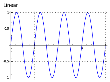 Time
Time-> 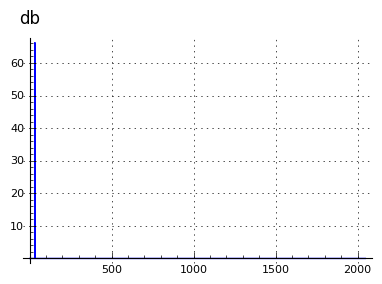 Frequency
Square wave:
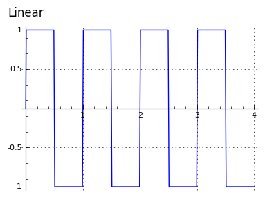 Time
Time-> 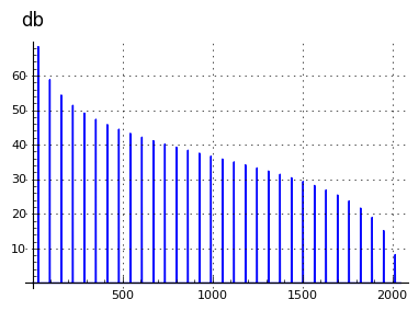 FrequencyFigure 5: Comparison of sine and square wave spectra.
Here's what this kind of interference looks like:

Figure 6: Spectrum display of locally-generated interfering signals.
It's not easy to create an antenna that receives only desired signals and rejects the noise of modern, high-speed electronic circuits, but it can be done.
PLSDR Detailed Description
Basic operation
- Because many of the preliminaries have been covered above in the installation section, I'll assume you have a radio device configured and ready for connection to PLSDR. So:
- Connect the radio device to your computer and to an antenna.
- Launch PLSDR, go to the Control ... Device item and select the device with a name similar to your device.
- Item (2) should cause PLSDR to open communication with your device and, if the transaction/setup is successful, the Start/Stop button at the upper right will be enabled.
- A transaction/setup failure is indicated by an inactive Start/Stop button and the message "No radio device detected" on the program's status line.
- If item (2) fails to enable the Start/Stop button, this might be caused by having chosen the wrong item in the Device list, lack of a suitable installed driver, or the possibility that your device is not supported by Gnuradio's driver scheme — see the "Troubleshooting" section below for some remedies.
- Click the Start/Stop button to begin radio data processing.
PLSDR offers a number of ways to change frequencies:
- Choose a frequency from the provided frequency list (at the tab marked "Frequencies" at the lower left).
- Spin your mouse wheel against any of the green frequency digits at the upper left.
- (Right-clicking a frequency digit zeroes all the digits to the right.)
- After clicking one of the frequency digits, one may use keyboard keys:
- "+" and "-" change frequency by 100 Hz.
- Left and right arrow keys change by 1 KHz.
- Up and down arrows change by 10 KHz.
- Page Up and Page Down change by 100 KHz.
- Insert and Delete change by 1 MHz.
- Double-click a frequency (i.e. location) on the spectrum display to center that frequency in the receiver's passband (the vertical red line).
- Drag your mouse cursor horizontally on the spectrum display to change frequencies or ...
- Drag vertically to change the position of the decibel trace.
- Spin your mouse wheel against the spectrum display to expand ("zoom") the frequency scale or ...
- While holding down the keyboard Ctrl key, spin your mouse wheel in the same way to expand the vertical decibel scale.
- Right-click the spectrum display to restore it to its default frequency width and decibel height.
The Waterfall display (lower left tab marked "Waterfall") shows a time record of past received signals. Its displayed colors may be adjusted with the mouse wheel. The speed of the waterfall display is determined by the spectrum display's Rate FPS setting described below.
The Control tab at the right provides many configuration options:
- For devices with more than one antenna port, the Antenna list provides a way to change ports.
- The Mode list includes AM, FM, WFM, USB, LSB, CW/U, and CW/L.
- AM stands for Amplitude Modulation which, apart from Morse code, is the oldest form of radio communication.
- WFM, used in FM broadcasting, is the wideband version of FM (Frequency Modulation), while the latter is used in point-to-point communications.
- USB and LSB stand for upper and lower sideband, variations on a very efficient communications method described more fully below.
- CW/U and CW/L are variations on USB and LSB with the presence of an audible tone to facilitate Morse code reception.
- The gain controls below the Mode list (from 1 to 4 in number) have different names and functions with different radio devices, and are defined by the radio device during initialization.
- The same is true for the "RF BW Hz" bandwidth control — its range and properties are defined by the radio device.
- The Squelch control serves a classic function in radio communications — it mutes the audio when incoming signals fall below a chosen level. Remember this control and its function if the receiver should inexplicably go mute.
- The Averaging control uses a moving-average algorithm to smooth out the noise in the spectrum display. It's an efficient way to reveal signals that might otherwise be buried in noise.
- The AGC (Automatic Gain Control) list includes various strategies to automatically control the receiver's gain. Of particular interest is SW/S, a slow-AGC mode that is useful when receiving single-sideband signals.
- The IF BW (Intermediate-Frequency Bandwidth) options buttons change the receiver bandwidth for different conditions.
- The FFT Size control changes the array size for the Fast Fourier Transform that powers the spectrum display. Larger arrays produce more detail but require more time to produce a spectrum. If the receiver's audio begins to break up or if the spectrum display seems unacceptably slow, decrease the size of the FFT array.
- The Rate FPS control selects the rate at which new spectra are generated. In some cases slower rates may prevent the computer from being overloaded with work.
The Configure tab contains these controls:
- Corr. PPM applies a user-entered frequency correction, with units of parts per million, to align the receiver's local oscillator with a frequency standard. As time passes available computer receivers are equipped with more accurate clocks, so this feature has become less important.
- Sample Rate is the rate at which data are generated and transferred to PLSDR from the radio device. This list is populated by the radio device during its initialization. Some receivers have severe limits on data rates, others are more powerful and flexible. There is also the issue of which kind of USB port (if used) carries the data. Older USB ports have limits on data rates, entirely apart from data rates the radio device might otherwise offer. In the event of erratic or slow receiver behavior, reduce this rate.
- Audio Rate is the rate at which audio data are transferred from PLSDR to your computer's audio system. This setting is more critical and less flexible than the receiver's sample rate, and only a handful of rates can be expected to work. A modern laptop/desktop will support a rate of 48,000 samples per second, while older equipment may be limited to 44,100 or 22,050 samples per second. Faster rates are better, but too high a rate may produce problems of its own.
- The Audio Device entry is initially blank (which invokes the system default audio device), but on some Linux distributions an entry of "plughw:0,0" may (by bypassing a slow audio protocol) produce better results than the default (meaning a blank entry). But some systems use unexpected numbers for this entry — to find out what the possible numbers are, run this command in a terminal session:
The aplay command output lists card numbers at the left and device numbers to the right. In an entry of "plughw:x,y", x = card number and y = device number. For one system that uses HDMI sound, after some experimentation I entered "plughw:1,10" to get the desired result. If you exit PLSDR using the "Quit" button, your choice will be saved for next time.$ aplay -l- The CW Base Frequency entry is a matter primarily of interest to radio operators able to interpret on-air Morse code. It specifies the frequency of the receiver CW passband center in Hertz.
- PLSDR's upconversion feature automatically applies a block-upconversion frequency (with a default of 125 MHz) to receiver tuned frequencies below a specified transition frequency (with a default of 24 MHz). This simplifies the use of block upconverter devices like the "HamItUp" device. When this feature is enabled the block-upconversion frequency is automatically applied to frequencies in the specified range, but the user must still throw the upconversion switch on the HamItUp device.
- The "Upc. Corr. PPM" entry applies a user-specified frequency correction to the particular case of an operating upconverter. The reason for this separate correction is because the upconverter device has its own clock, separate from that in the receiver device, and this clock may require a separate correction.
- The Offset Tuning feature addresses a problem common to most computer receivers — they produce what is called a "DC spike," a strong pseudo-signal at zero Hertz that in many cases can interfere with reception of weak signals. The offset frequency option deals with this by applying a small offset frequency to the receiver, in a way that doesn't degrade tuning accuracy or spectrum display, but that allows the receiver to operate at full sensitivity. The entered offset may be positive or negative but cannot exceed 1/2 the audio sample rate.
Frequency list
- PLSDR gets frequency information from user entries, but it also displays a default frequency spreadsheet that the user can edit to his own tastes.
- The spreadsheet is named
"frequency_list.ods"and is automatically installed in the user-data PLSDR directory (not the program directory) — which, by the way, will be located here:Linux:
/home/(username)/.PLSDR/frequency_list.odsWindows:
/users/(username)/.PLSDR/frequency_list.ods- The spreadsheet is LibreOffice compatible and contains columns of names, frequencies and comments.
- Although this specific spreadsheet has particular column names and related information, PLSDR will accept many variations. There's only one requirement: one of the columns must contain frequencies and a special heading that includes one of the tokens 'GHz', 'MHz', 'KHz', or 'Hz', (case insensitive) with frequency data in that column that corresponds to the provided unit.
- If the user prefers, PLSDR will accept a plain-text CSV (comma-separated values) file instead of a LibreOffice spreadsheet. The same format applies as above — any number of columns in any order, but one of them must contain frequencies and the special header described above.
- Finally, neither the spreadsheet nor the CSV file need have any particular name. The only requirement is that a user-provided spreadsheet have the ".ods" suffix, or a provided CSV file have a ".csv" suffix. If both kinds of file are in the user directory simultaneously, PLSDR will prefer the spreadsheet.
Language and architecture issues
- Python: PLSDR is written entirely in Python, a comparatively slow interpreted language.
- Python development is fast (no compilation required) but the resulting programs can sometimes be slow.
- For this program, the consequences of writing in Python are not very severe because the Python code assembles GnuRadio code blocks written in C and C++, and those blocks then run at a much higher speed than Python would be capable of.
- There are a few exceptions to the above description. The spectrum display code is entirely Python, fortunately this feature doesn't require much computer power to render.
- One advantage to Python is that the application's running code is also the source code for the project. This is particularly convenient for open-source projects like PLSDR.
- Operation on a Raspberry Pi: Earlier Raspberry Pi models couldn't handle the combined PLSDR/GNURadio processing load, but according to user reports, more recent Pi models manage this workload easily.
- Zero-Hz Spike: Most radio devices produce a "spike," a spurious signal, at zero Hz, and most software-defined radios have a way to deal with this. The usual remedy is to move the receiver's passband away from zero Hz by a small value and realign the frequency display to make this change transparent. PLSDR offers this option for those devices that need it (details above).
- Upconversion: Some radio devices use an upconversion scheme to extend their frequency coverage — the HamItUp device is an example. In this scheme, below a certain frequency, an accessory upconverter block-shifts frequencies into the base device's normal acceptance window (which normally extends from 24 MHz up to 1 or 2 GHz). This allows radio reception between 0 Hz and 24 MHz.
- Some SDRs require that the user manually enter a conversion frequency and throw a switch to enable upconversion. PLSDR has a user-selectable feature that automatically includes the conversion frequency for tuned frequencies below a set limit. The user must still throw a hardware switch (can't automate that).
Radio Device User Configuration
- At the time of writing the author only has four computer radios (HackRF One, NooElec, RTL-SDR and SDRplay), all of which are known to work with PLSDR simply because they were available for testing. PLSDR includes a much longer list of radio types, but for lack of hardware, no practical way to verify their operation.
- The longer list of untested radio names and invocation strings is derived from Internet searches, but since no direct tests have been performed, these entries are of questionable value.
- For radios in PLSDR's list that have not been tested, users are encouraged to edit one of PLSDR's source files to accommodate new information as it becomes available. Specifically, in the PLSDR.py file, there is a Python dictionary named "device_dict" near the top of the file. This dictionary's entries look like this:
'display name' : 'invocation string',- The key to successful changes to existing entries is to enter and test a different (working) invocation string, the item at the right. For a radio not included in the default list, one may add a completely new entry as shown above — a display name and invocation string, both quoted as shown and followed by a comma.
- As new information becomes available, this dictionary's contents can and should be edited to reflect that new information. And for changes that work, that successfully communicate with radios, the author would appreciate hearing about these changes so others may benefit (use the message board link at the top of this page, or click here). Thanks!
GnuRadio Companion Scripts
- The author used GnuRadio Companion (the GnuRadio design environment) a great deal during this project's development phase. The resulting scripts aren't completely synchronized with the block configuration in the project any more, but readers might find them interesting. The ZIP archive contains both transmitter and receiver modules of various kinds.
PLSDR was developed using this general strategy:
- Each receiver mode was prototyped using a powerful GnuRadio graphic development environment named "GnuRadio Companion" (hereafter GRC).
- In GRC, functional blocks can be moved about and connected in different ways using a clever GUI interface, then tested in a live interactive environment.
- Once the prototyping phase was complete, the design was converted into PLSDR project code by importing GnuRadio and other essential libraries to support the design strategy commonly used in GnuRadio projects, then writing versions of the GnuRadio functional blocks from the prototyping phase.
- The design was then tested and fine-tuned in a native Python environment to determine whether the prototype scheme could be further optimized and refined.
- Special blocks were written to allow extraction of data from the GnuRadio block scheme to support custom-written spectrum and waterfall displays.
For lack of useful online documentation the single-sideband decoder that's now part of PLSDR required a significant effort to design, although it probably shouldn't have. But first, a little history.
Single-sideband radio transmission and reception is a clever and efficient strategy to squeeze as much communications capability as possible out of a given amount of radio spectrum and transmitter power.
From the early days of radio, the original voice transmission mode was AM, Amplitude Modulation, which has this spectrum (the horizontal dimension has units of frequency, not time):
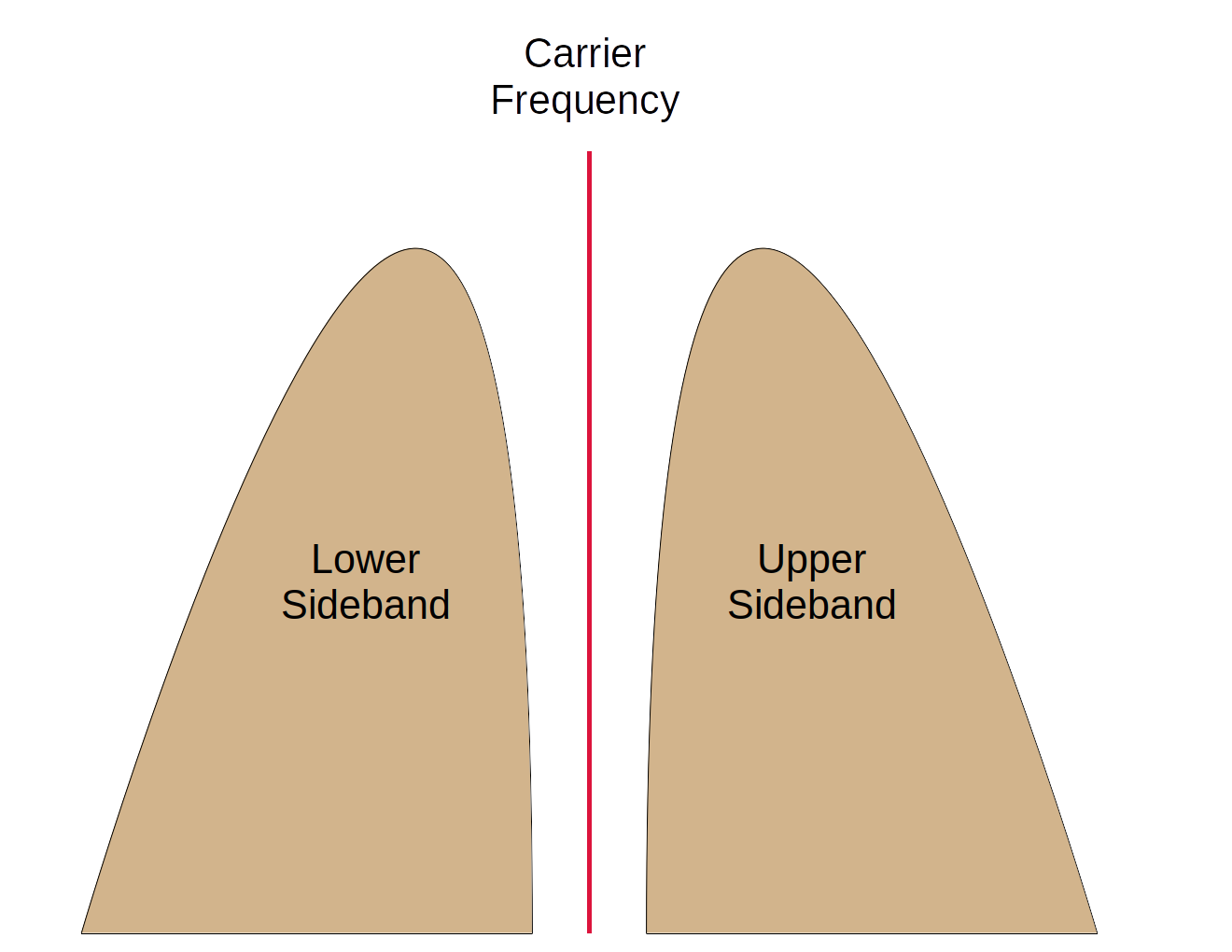
Figure 7: Amplitude Modulated radio signal
Because the sole purpose of the signal is to transmit the information in the sidebands, it occurred to workers in the field that this purpose could be served by transmitting only one of the sidebands, eliminating the carrier and the other sideband (the carrier signal, essential for decoding the remaining sideband, is restored in the receiver). After some clever engineering work, the Single-Sideband (SSB) method was devised. A single-sideband signal looks like this:
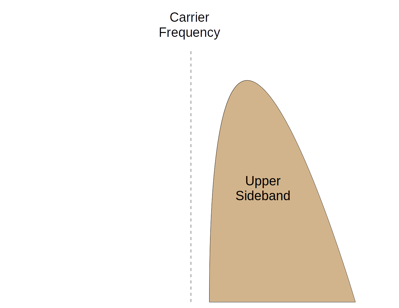
Figure 8: Single-Sideband radio signal
In Figure 8 the carrier and one sideband have been eliminated (the carrier's location is marked in Figure 8 but it's not actually present), resulting in a substantial saving in transmitter power and spectrum use.
When transmitting single sideband, one wants to save power and limit spectrum use by eliminating the carrier and one sideband, as in Figure 8. When receiving, one wants to completely filter out the unused sideband region of the receiver passband to limit interference from adjacent transmitters. The technical methods for transmitting and receiving single sideband signals are similar but not identical.
There's a crude method to create single-sideband signals that involves use of filters — one bandpass filter for each sideband. But this method is generally unsatisfactory, slow in operation, inflexible and complex. In radio design, using a bandpass filter to create a single-sideband signal is usually an acknowledgment of defeat.
In the PLSDR design phase, because of my use of Python and its limited speed, I sought the simplest, most effective and least processing-intensive sideband decoding method. I understood the theory and the mathematics, but to save time I decided to search online for methods other GnuRadio users might have posted.
After several hours of research, I came to an astonishing conclusion — of the dozen or so online examples of GnuRadio single sideband creation and decoding methods, not one of them was even remotely correct. All the authors were confident in their methods, and each was entirely wrong. At the time I write this, there isn't one correct single sideband creation or decoding method posted online. Don't get me wrong — there are plenty of published single sideband methods created using GnuRadio's tools and then published in various online forums, but every single one of them is flat wrong (hover-footnote).
In my favorite online example, one person posted a request for assistance with an SSB decoder design he couldn't get working, and another apparently more experienced designer explained that the beginner's design couldn't possibly work — it needed to be more complex. The more experienced hand then showed his own much more complex design which, apart from being five times more complicated than necessary, can't decode single-sideband signals any better than the method posted by the beginner (I know, I assembled and tested it). And in a surreal touch, the experienced designer fed the real component of his decoder's complex output to one stereo audio channel, and the imaginary component to the other, as though those listening to the audio would be able to distinguish between them.
At this point the more technically experienced among my readers will want me to show my design, which actually works. How did I create and test it?
First, a word of warning — the only meaningful validation for a single sideband receiver is to test it against a properly configured single sideband transmitter, preferably one emitting a voice signal. There are any number of online examples of decoders tested using noise sources — apparently the authors didn't realize that a noise source is very likely to confuse the test and the tester — it's common for a noise-based test signal to mix the upper and lower sidebands, then put both of them on one side of a spectrum display, creating the illusion of success.
In my tests I used the GnuRadio design facility to create a single sideband transmitter, which played a voice podcast on one computer equipped with a radio signal emitter (HackRF), then tested my receiver designs against that signal source on a separate computer and radio device. I included the all-important step of deliberately switching the transmitter and receiver to opposite sidebands to verify that no signal was getting through — something not one person who posted SSB designs online apparently thought to try, or knew how.
But enough history — let's discuss some theoretical issues. The key idea in modern single-sideband encoding and decoding is to take advantage of complex (in the mathematical sense) signals that have components in quadrature (meaning a two-component vector whose components differ by 90°). The conventional terminology for this kind of signal is I/Q, I (In-phase) being the real part and Q (Quadrature) being the imaginary part of a complex signal.
The more advanced single-sideband designs use a phasing method, one that takes advantage of the phase relationship between the I and Q signals to mathematically suppress the unwanted sideband. Here's a classic example:
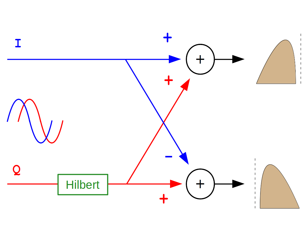
Figure 9: Phasing method for sideband suppression
Now think about this. If we have two waveforms that always differ by 90°, and if we know that the relationship between the components is reversed on one side of zero Hertz compared to the other (for positive frequencies, Q lags I in time by 90°, for negative frequencies, Q leads 90°), to eliminate one sideband all we need is a special device that adds 90 more degrees of phase shift to all frequencies of interest. That would produce 180° of phase shift on one side of zero Hertz, or to put this another way, the two waveforms would be in precise opposition there. Because this special phase shift is applied to only one of the two I/Q components, if the resulting components were added together the result would be zero amplitude on one sideband, and a doubling of amplitude on the other, at all frequencies. That's an ideal outcome, one that can't be approached using a bandpass filter.
So what is this fantastic device that adds exactly 90° of phase shift to all frequencies and makes this all possible? It's called a Hilbert transformer. It's not possible to create an ideal Hilbert transformer (whose perfect behavior can only be described mathematically), but practical embodiments are pretty good. Again, this device has the property that it adds 90° of phase shift to all frequencies, not just one. This means it can be configured to completely eliminate one sideband of a complex, wide-bandwidth signal.
But rather than try to use words to explain this, I offer this JavaScript app, which shows the process graphically:
USB Frequency: Hz
Figure 10: JavaScript single-sideband filter app
Notes:
- The I (In-phase) trace is the real part of the complex incoming radio signal.
- The Q (Quadrature) trace is the imaginary part of the signal — it always differs by 90° from the I trace, either leading or lagging in time.
- For positive frequencies, Q lags I in time by 90°, as shown with the default settings above.
- For negative frequencies, Q leads I in time by 90° — test this by moving the frequency slider to a negative frequency.
- The Hilbert signal always lags Q in time by 90°, regardless of frequency. This is important to understand.
- The Output trace is the sum of I and Hilbert, as shown in Display B above.
- Because the relationship between I and Q depends on frequency, and because Hilbert always lags Q regardless of frequency:
For positive frequencies, Q = I + 90° and Hilbert = Q + 90° as shown in Display A with default settings, therefore Hilbert is 180° out of phase with I, and the Output sum of the I and Hilbert signals is zero, as shown in Display B with default settings.
For negative frequencies (move the frequency slider left to a negative setting), Q = I - 90° and Hilbert = Q + 90° as shown in Display A with a negative frequency setting, therefore Hilbert is exactly in phase with I, and the Output sum of the I and Hilbert signals is twice the normal signal amplitude, as shown in Display B with a negative frequency.
- Switching between upper and lower sidebands is accomplished by reversing the sign of the Hilbert signal that's applied to the Output adder (try it above — click the USB checkbox).
- In the above app, the positions of the I and Hilbert traces are slightly offset vertically so the reader can see both traces when they're in phase. This offset isn't part of the real process.
After reflecting on these issues and, because of a limitation in the GnuRadio Hilbert filter design, I was obliged to create an unnecessarily complex (notes below) but effective single-sideband decoding filter that, in its final form, looks like this in GnuRadio Companion (and in PLSDR):
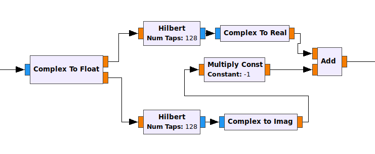
Figure 11: GnuRadio Companion SSB decoder diagram
Notes on Figure 11:
- Because the GnuRadio Hilbert block isn't an optimal design, this filter is more complex than necessary — I was forced to to use two Hilbert transformers where only one is actually needed.
- This results from the fact that this real-world embodiment of the Hilbert transformer doesn't just shift phases by 90°, it also creates a time delay, and to avoid spoiling the timing of the design, an identical time delay must be included in the other branch of the decoder. The existing Hilbert transformer design provides this essential time delay as one of its two outputs, but if the design requires two input pathways (one for I, one for Q), then the time-delay value must be acquired from a separate Hilbert transformer.
- So in Figure 11, one Hilbert transformer actually performs the intended 90° phase shift, while the other provides the exact time delay of the active device to keep the system synchronized.
- It would be nice if these two signals emanated from a single GnuRadio Hilbert block, one that accepted a complex input — that would eliminate some unnecessary complexity in this design.
- To me personally, a perfect GnuRadio Hilbert block would in some ways be the opposite of the existing one. The perfect Hilbert would accept a complex input, thus eliminating my "Complex to float" block at the left, and it would produce two float (i.e. non-complex) outputs, thus eliminating my "Complex to Real" and "Complex to Imag" blocks at the right.
- The purpose of the "Mult" block is to reverse the sign of one of the inputs to the adder at the right, which has the effect of switching from one sideband to the other.
There are obviously any number of ways to create and decode single-sideband signals, since we're surrounded by radios that do this routinely, but as I write this the Internet has zero usefulness as a research resource on this topic. Again, I can't believe the number of people I located who tried to design an SSB encoder or decoder, utterly failed, then posted their results on the Web just as though they had succeeded. I realize this group has two sub-populations — those who knew their designs didn't work, and those who, because of defective testing procedures, sincerely believed their designs worked. But both groups posted their results online without hesitation.
As I write this, there isn't a single working GnuRadio SSB encoder or decoder design posted online. Tomorrow there will be one.
Here's another JavaScript app (originally written for another article) that assists visualization of the complex I/Q signals used in modern radio work.
Figure 12: Interactive JavaScript I/Q exploration appletInstructions and suggestions for Figure 12:
- Enable real-time animation by selecting the "Animate" checkbox.
- Rotate the 3D graph by dragging your pointing device on its surface, zoom with your mouse wheel.
- Try enabling/disabling the provided options and entering different frequences and rates.
- A set of example Configuration State buttons is provided to show various aspects of I/Q sampling:
- The State A example forces the 3D display into a flat, old-style 2D oscilloscope display without I/Q sampling, just to provide a contrast with the newer methods. After clicking "State A", rotate the graph with your pointing device to bring the I/Q elements back into view.
- The State B example shows the phase relationship between I and Q for the case of a positive frequency. In this case, Q lags I by 90° or $\frac{\pi}{2}$.
- The State C example shows the phase relationship between I and Q for the case of a negative frequency. Notice that the only change between this example and State B is in the phase of Q, which tells us that an old-style mixer without I/Q sampling would not be able to distinguish between a positive and negative frequency.
- The State D example shows a time animation of a negative frequency vector. To see the contrast between negative and positive frequency, change the sign of the carrier frequency and notice that the vector's direction of rotation reverses.
- Remember that the meaning of "clockwise" and "counterclockwise" depends on one's point of view. For example, the default animation appears to show a clockwise rotation for a positive frequency, but this is so only because of the default graph point of view, located to the right of the graph. But the clockwise/counterclockwise convention applies only when looking toward a future time, i.e. from a position at the left of the graph, as in the State D example.
- To speed up / slow down the animation rate, increase / decrease the value of "Anim. Step."
- To see this display in true 3D, select the "3D" checkbox and grab a pair of red/cyan "Anaglyphic" 3D glasses.
- It's my hope that this applet will provide a memorable visualization of the details of I/Q sampling, to help the reader acquire an intuitive sense of how and why it works.
This page has two goals — introduce an advanced SDR program, and teach a little radio theory. I hope it succeeds in both efforts.
I already have a list of future changes to PLSDR. One will be a way to record raw I/Q data, that shouldn't be difficult at all. Another will be a way to remotely control PLSDR using a network connection. That might be a bit more difficult, primarily having to do with choosing a rational, understandable protocol for the link.
It's my hope that this program — and this page — will help people better understand mathematics and modern technology, as well as meet people's practical needs.
PLSDR is © Copyright 2020, P. Lutus and is released under the GPL.
PLSDR is also a GitHub project: https://github.com/lutusp/PLSDR/
- 2020.04.25 Version 2.0. Now that GNURadio 3.8 is generally available, this version uses Python 3.+ and GNURadio 3.8+. While converting, fixed a few small bugs.
- 2018.05.22 Version 1.9. Changed default audio device to "" (which invokes the system default) after user problems with the earlier value. It turns out that the original default of "plughw:0,0" is only recognized by certain Linux distributions and causes a failure in others.
- 2018.04.06 Version 1.8. Substantially revised the program code and Windows launch scripts to deal with certain annoying Windows behaviors. PLDR can now be installed in any convenient location on a Windows system and it will run correctly.
- 2018.04.01 Version 1.7. Changed the slow-AGC time constant to a more meaningful value.
- 2018.03.31 Version 1.6. Changed to a more robust program path detection method based on user feedback.
- 2018.03.31 Version 1.5. Based on user feedback, corrected an error in the device definition dictionary "device_dict".
- 2018.03.30 Version 1.4. Caught and corrected a potential divide-by-zero condition.
- 2018.03.30 Version 1.3. Solved a sensitivity problem with the squelch feature.
- 2018.03.30 Version 1.2. Changed the installation procedure to reflect GitHub project conventions (added a "requirements.txt" file).
- 2018.03.29 Version 1.1. Changed to a power-law volume control method (many different devices with widely varying volume levels).
- 2018.03.29 Version 1.0. Initial Public Relase.
| Home | | Ham Radio | | | | Share This Page |
