
 Share This Page
| Home | | Sailing | | Alaska 2013 | | | Share This Page |

Copyright © 2013, P. Lutus. All rights reserved. Message Page
| Prior years: |
Alaska 2002 |
Alaska 2003 |
Alaska 2004 |
Alaska 2005 |
Alaska 2006 Alaska 2007 | Alaska 2008 | Alaska 2009 | Alaska 2010 | Alaska 2011 Alaska 2012 |
(double-click any word to see its definition)
This article describes the behavior of water flowing into and out of bays and channels, a matter of much interest to sailors. Most of my Alaska articles aren't technical, but this one certainly is. To avoid losing any readers who don't like seeing equations, I've divided this article into two sections. The first describes the dynamics of water flow in everyday terms and offers some commonsense tips for sailing and boating activities. The second section provides a full technical background for the article's conclusions.
This article expands on my earlier work on this topic, adding more information and improving the mathematical treatment.
Understanding tidal dynamics in channels and bays requires just a little intuition, and this article includes an interactive model to help the reader's intuition along. The water level in a bay changes more or less in step with ocean tides, usually somewhat delayed, in a way determined by the bay's size and its entrance channel's resistance to water flow. When flow resistance is present, the bay's high and low tide times are usually delayed compared to the ocean times, and the tidal range within the bay is smaller as well.
For large bays and narrow connecting channels, the timing of high and low tides within the bay can be delayed as much as three hours past the time of the ocean's highs and lows. For such a bay, the magnitude of the tides is greatly reduced compared to the ocean.
In the interest of safety, boaters need to know slack water times in a bay's entrance channel. This article and its graphic model will help the reader learn how to estimate slack water times for channels that don't have published predictions, and understand why channel and bay waters behave as they do.
(Click image to start/stop animation.)
| Model Controls: | r: | c: | k: |
Note: If you can't see the model above, or if it's not working correctly, you may want to update your browser. Consider these options:The third choice is the least satisfactory — Chrome and Firefox are much better browsers.
- Install Google Chrome.
- Install Mozilla Firefox.
- For Windows users, install a newer version of Microsoft Internet Explorer if you can (Windows XP users don't have this option).
Figure 2 is a mathematical model showing the interplay of tidal flows between the ocean and bays of different sizes, by way of channels with varying resistance to current flow (the model itself is fully described in a later section). Three user-adjustable variables control the model:
- r: The channel's resistance to water flow.
- c: The bay's capacity (or volume).
- k: A factor describing how much fresh water flows into the bay.
Feel free to experiment with the model. By adjusting the controls, the reader can adjust the bay's tidal dynamics to match most bays one might encounter in real life, including those with fresh water inflows.
A little experimenting with the model should lead the reader to these conclusions:
- Small bays with wide entrances tend to have tides much like the ocean's tides — similar timings and heights, slightly delayed in time. To see this in the above model, set c at or near zero.
- Larger bays (increased values for c above) and bays with narrow, confining channels (larger values for r), have tidal highs and lows that are delayed in time past the ocean's tides, sometimes as much as three hours, and the bay's tidal extremes are smaller than those seen on the ocean.
- The largest bays, and those with the narrowest entrance channels, tend to have a nearly constant water level roughly equal to mean sea level, and channel slack water times can be as much as three hours after ocean high and low tide times. To see this in the above model, set c = 3.
- With one exception described below, the connecting channel's slack water times are always later than the times of ocean high and low tide, and those slack water times typically match the times of the bay's high and low tides.
- The exception is a bay that has fresh water inflows (increased values for k above). Such a bay has a higher average water height than the ocean, and the channel's slack water times are changed compared to bays without fresh water inflow — high slack water is earlier than expected and low slack water is later. To see this in the above model, set k to values greater than zero.
- For a bay with high amounts of fresh water inflow and a narrow entrance channel, the water in the bay tends to be a mixture of fresh and salt water. Such a bay is called a lagoon.
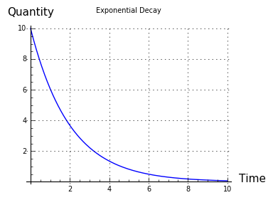 Figure 3
It's important to understand that this model is somewhat idealized compared any any real bay/channel system in nature (a scientist would call it a "first-order appproximation"). The model accurately portrays the physics of water, but only for a hypothetical system having a channel whose cross-sectional area doesn't change with water height, and whose resistance doesn't change with water flow rate (both of which do change in a real channel).
Exponential Decay
But the model does show an important rule that's common to many physical systems — water flow, electrical current flow, gas flow between connected reservoirs, heat flow from a hot to a cool object, and others — and the rule is the rate of flow is proportional to the remaining difference in quantity (this rule is named exponential decay). What this means is that, as water, or electrical current, or gas, or heat energy, flows from one location to another and equalizes the quantities, that has the effect of proportionally reducing the rate of flow.
If you think about this, it may occur to you that, as the difference in quantity approaches zero, the flow rate declines in proportion, so in principle the rate should never equal zero, and the two quantities will never become equal. And that's right — in physical systems like this, where the exponential decay rule applies, the two connected quantities only ever approach equality, regardless of the amount of time (Figure 3).
In an ocean/channel/bay system, exponential decay is shown by the fact that the bay's water level is constantly changing to match the ocean's water level — rising when the ocean is higher, descending when it's lower, and unchanging when the levels are the same. Consistent with the exponential decay rule, notice that the current velocity is proportional to the difference between the ocean and bay water heights (this is clearly shown by the model in Figure 2). So the velocity of the channel current represents a rate of change in the bay's water level — higher rate of change, more velocity — and that rate of change is proportional to the difference between the ocean and bay water heights.
Summary
The most concise summary of this section might be:
- Bay entrance slack water times are typically after the time of ocean high or low tide, sometimes long after for big bays.
- Channel slack water time is normally the same as the bay's high and low tide times (not the ocean's times). This is clearly shown by the model in Figure 2.
- A bay's mean water level is normally the ocean's mean level, unless fresh water flows into the bay, in which case the bay mean level is higher than the ocean mean level.
These are just a few easily remembered principles, derived from applying mathematics to reality. In the next section, we show the mathematics.
The first section of this article allows readers to view a graph of a differential equation with adjustable parameters. A differential equation is one that includes derivative terms, terms that describe rates of change. Such an equation differs from an ordinary algebraic equation in that its result varies as a function of one or more of its input parameters. Another way to say this is that a differential equation models a changing system.
Analysis
Because tidal current flows are an example of exponential decay, let's start with a simple exponential-decay differential equation. This equation is widely applied to problems that involve a rate of change depending on the remaining difference between two levels:
(1) $y(t) + r\ c\ y'(t) = m$Where:
- y(t) = an unknown function with respect to time.
- y'(t) = first derivative of y — meaning a rate of change in y — with respect to time t.
- t = time, usually seconds.
- r = In an electrical circuit, resistance to electrical flow in ohms. In a tidal problem, resistance to water flow.
- c = In an electrical circuit, capacitance in farads. In a tidal problem, the capacity (volume) of a bay.
- m = in an electrical circuit, source voltage. In a tidal problem, ocean water height outside a bay.
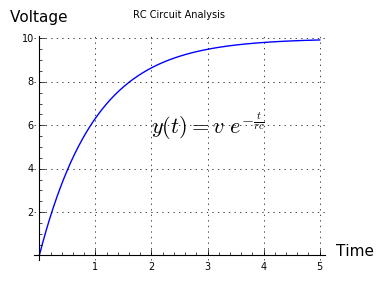 Figure 4
The solution for the above terms is:
(2) $ \displaystyle y(t) = m e^{-(\frac{t}{r c})} $Where $e$ = the base of natural logarithms.
Equation (2) is the dimensionless, and therefore most universal, form of the canonical exponential decay equation. Because it's dimensionless as shown, terms can be added to the equation to get it to model a number of physical systems. For example, in an electrical resistor-capacitor circuit, in which a switch connected to voltage v is closed at time zero, the equation would look like this:
(3) $ \displaystyle y(t) + r\ c\ y'(t) = v$The solution in this case is:(4) $ \displaystyle y(t) = v\ e^{-(\frac{t}{r c})} $As it happens, this exponential decay function applies equally, and almost identically, to tidal problems, electrical circuits, gas flow between reservoirs, heat flow and many other natural systems. Such equations demonstrate the universal nature of mathematical physics — a single equation may model a basic principle having any number of expressions.
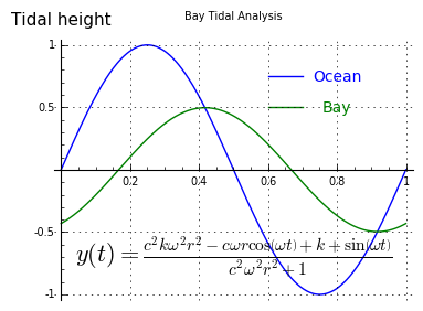 Figure 5
Continuous Decay Function
So far, we've shown a system that models an exponential decay system that begins at zero and ends at a predetermined endpoint v, such as one might find in an electrical engineering textbook. Now let's add some terms to make the outcome resemble continuous tides and tidal currents.
(5) $ \displaystyle y(t) + r\ c\ y'(t) = sin(\omega t) + k$Where the new/redefined terms are:The solution in this case is:
- $\omega = 2 \pi f$, i.e. angular frequency in radians/second.
- f = tidal frequency, Hz.
- r = flow resistance in entrance channel.
- c = bay capacity (volume).
- k = term for constant water flow into system.
(6) $ \displaystyle y(t) = \frac{c^{2} k \omega^{2} r^{2} - c \omega r \cos\left(\omega t\right) + k + \sin\left(\omega t\right)}{c^{2} \omega^{2} r^{2} + 1} $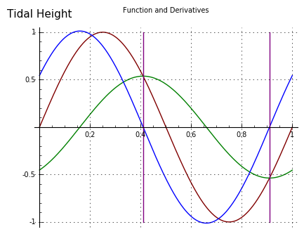
- $ \displaystyle y(t) = sin(\omega t)$
- $ \displaystyle y(t) = \frac{c^{2} k \omega^{2} r^{2} - c \omega r \cos\left(\omega t\right) + k + \sin\left(\omega t\right)}{c^{2} \omega^{2} r^{2} + 1} $
- $ \displaystyle y(t) = \frac{c \omega^{2} r \sin\left(\omega t\right) + \omega \cos\left(\omega t\right)}{c^{2} \omega^{2} r^{2} + 1} $
Figure 6The model presented as Figure 2 above is built around equation (6), a relatively simple tidal model with one cyclical term. Earthly tides in nature, of course, have at least two terms, one for the moon and one for the sun, and often must include other terms to account for landscape and similar factors. As it turns out, equation (6) can be written to accommodate any number of terms if managed carefully, and still retain the advantages of its analytical form.
Derivative Form
For the nonmathematicians among my readers, the advantage of the analytical form is that it can be symbolically manipulated to produce additional results. For example, the first derivative of equation (6) is:
(7) $ \displaystyle y'(t) = \frac{c \omega^{2} r \sin\left(\omega t\right) + \omega \cos\left(\omega t\right)}{c^{2} \omega^{2} r^{2} + 1} $Equation (7) can be used to easily compute the times of slack water in the modeled bay and channel — its zeros are the slacks in the system, the times of no channel current (Figure 6, vertical lines).
Limitations
Equations (6) and (7) are only meant to show some important properties of tides, in particular the relationship between tides and currents in bays, but even when written to accommodate more tidal terms, they're too simple for use in real tidal forecasting. Another way to say this is that these equations, which tell us something important about every tidal system, aren't exactly right about any of them.
In practice, tidal forecasting relies on observations of nature (field measurements), then the observations are turned into a basis for prediction through a mathematical regression method known as Fourier analysis. Tidal forecasting shows the limitations of a purely analytical treatment of nature. For many natural systems, we can't accurately model nature's behavior with closed-form equations like those above, instead we must turn direct observations into numerical forecasts, without trying to directly apply basic physical principles to the process.
The value of equations like those in this section is that they show first-order properties of every tidal system, even though specific tides must nearly always be modeled numerically. The conceptual distance between these equations and a real tidal system only supports Albert Einstein's well-known dictum, "As far as the laws of mathematics refer to reality, they are not certain, as far as they are certain, they do not refer to reality."
- The majority of the mathematical analysis, and the graphics for this article, were created using Sage, a free, open-source mathematical environment.
- Differential Equation — an equation for an unknown function that includes derivative terms, often one that models a dynamic system like tides. Some differential equations have closed-form solutions, others must be evaluated using numerical methods.
- Theory of Tides — a description of the physics behind tides.
- Fourier Analysis, a.k.a. harmonic analysis, a rich field of mathematical analysis with many aspects, including the ability to transform time-domain functions into equivalent frequency-domain functions and the reverse.
| Home | | Sailing | | Alaska 2013 | | | Share This Page |