Share This Page
| Home | | Mathematics | | | | Share This Page |
Copyright © 2022, P. Lutus
This is the JavaScript version of PolySolve
Most recent update to this page:
Most recent update to polysolve.js:
Note: In this article, footnotes are marked with a light bulb over which one hovers.
For a given data set of x,y pairs, a polynomial regression of this kind can be generated:
$ \displaystyle f(x) = c_0 + c_1 \, x + c_2 \, x^2 + c_3 \, x^3 ... $In which $c_0,c_1,c_2 \, ...$ represent coefficients created by a mathematical procedure described in detail here.
In this regression method, the choice of degree and the evaluation of the fit's quality depend on judgments that are left to the user. It is well known about this class of regression method that an effort to squeeze more correlation out of the algorithm than the data can support will sometimes produce an out-of-control function that, although it matches the data points, wanders wherever it pleases between those points. Therefore, a "good" (approaching 1.0) correlation coefficient is not enough to assure a well-behaved or meaningful function. Decisions about a result's appropriateness is more a matter of judgment than mathematics.
A "perfect" fit (one in which all the data points are matched) can often be gotten by setting the degree of the regression to the number of data pairs minus one. But, depending on the nature of the data set, this can also sometimes produce the pathological result described above in which the function wanders freely between data points in order to match the data exactly.
For those seeking a standard two-element simple linear regression, select polynomial degree 1 below, and for the standard form —
$ \displaystyle f(x) = mx + b$— b corresponds to the first parameter listed in the results window below, and m to the second.
This regression is provided by the JavaScript applet below. To enter new data, type data pairs into the upper window (or paste from the system clipboard by pressing Ctrl+V), then press "Solve." To change the degree of the equation, press one of the provided arrow buttons.
NOTE: When using double-precision variables (as this program does), polynomials of degree 7 and above begin to fail because of limited floating-point resolution. The only practical remedy for such a case is to decrease the polynomial degree, regardless of the size of the data set (detailed explanation here). But in general, for problems requiring more than 7 coefficient terms or that show unsatisfactory results using this method, there are alternative regression methods including splines, and for periodic data sets, Fourier methods often produce excellent results.
Data Entry Area: Select: Ctrl+A | Copy: Ctrl+C | Paste: Ctrl+V
Chart Area:
Reverse Degree: 99 Results Area:Select: Ctrl+A | Copy: Ctrl+C | Paste: Ctrl+V
Table Generator:Select: Ctrl+A | Copy: Ctrl+C | Paste: Ctrl+V
Start: End: Step: Decimals: Exponential
First, if this program's results don't conform to user expectations, be sure to read the Technical Notes and Limits section below.
Each of the above data windows can deliver or receive data by way of the system clipboard:
- To paste from the system clipboard into a data window, click the window, press Ctrl+A (to overwrite existing content), then press Ctrl+V (paste).
- To copy from a data window, click the window, press Ctrl+A (to select all the data), then press Ctrl+C (copy).
- Having learned how to copy and paste to/from the system clipboatd, you can share this program's results with other programs, and other programs' data with this program.
- To acquire a graphic copy of the generated chart, press the "Graphic" button at the bottom of the chart display. This will create a graphic version of the chart in a separate window. Then right-click the graphic and choose "Save ..." or "Save as ..." or "Save Image as ...", depending on which browser is in use.
This JavaScript program replaces an earlier Java program with the same purpose. This recoding is meant to make this program more robust and portable. To use the earlier Java version, click here.
This section is meant for those needing a more portable and flexible polynomial data fit solution. It turns out that the polynomail regression method is available in most environments, and in modern Python it requires only a few lines of code. Here are some examples (these programs are released under the GPL):
Simplest Python Example
This example shows how one can use a modest amount of Python code to acquire a polynomial data fit and plot a result. Options:
Click here to see and download the Python program in plain-text form.
Click here to see a more readable (not to say beautiful) syntax-highlighted Python listing.
Notice in the above Python listing that the mathematical heavy lifting is carried out by just a couple of lines of Python (because the detailed algorithm is now enclosed in the numpy Python library):
# perform regression

def polyregress(xdata,ydata,degree):
  return numpy.polynomial.polynomial.polyfit(xdata,ydata,degree)
Example Chart
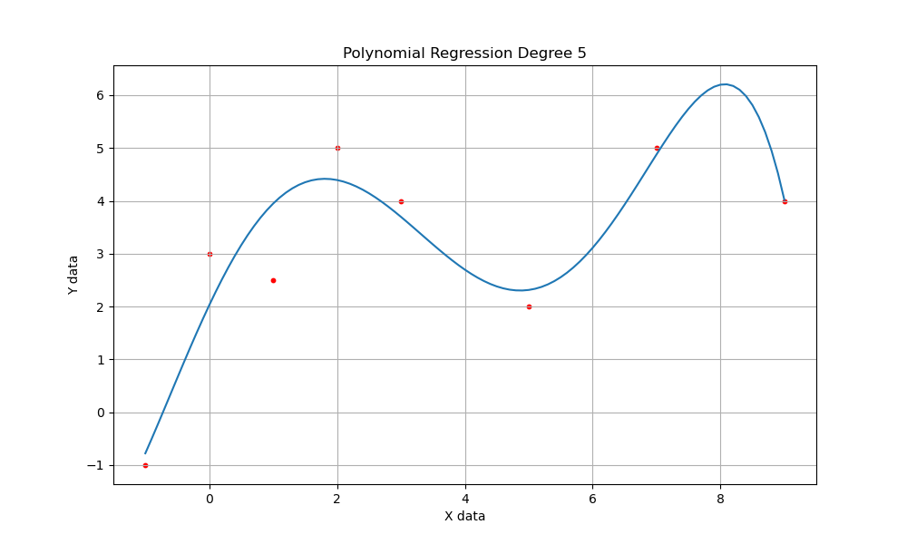
Here's an example chart generated by the above Python program, using the example data set from the JavaScript application above. To get this result from the Python program, users must install the Matplotlib Python library:
Older Python Example
I also have an older Python command-line program that produces the same results as the JavaScript and Python examples above. Because this program predates the ready availability of Python polynomial regression libraries, the polynomial-fit algorithm is included in explicit form. Click here to list and/or download the program. To use it, simply download it, make it executable and follow its instructions. Here's a test result that should agree with the above example result for a degree 5 polynomial:
$ echo "5 -1 -1 0 3 1 2.5 2 5 3 4 5 2 7 5 9 4" | ./polyregress.py -
Computer numerical processing imposes some limits on this regression method. Details:
A typical computer floating-point number can resolve about 15 decimal digits (see IEEE 754: floating point in modern computers), due to a double-resolution 52-binary-bit mantissa, and this conversion to a decimal equivalent:
For two number bases $A$ and $B$: \begin{equation} nd_B = \frac{nd_A \log(A)}{\log(B)} \end{equation} Where:
- $A,B$ = number bases, example 2 and 10.
- $nd_A,nd_B$ = number of available digits in $A$ and $B$.
So, for an IEEE 754 double-precision variable with a 52-bit mantissa:
\begin{equation} \frac{52 \log(2)}{\log(10)} = 15.65\, \text{base 10 digits} \end{equation}- When multiplying computer floating-point numbers, one multiplies the mantissas and adds the exponents, thus 2.0 * 107 times 3.0 * 10-7 = 6.0. No problem here.
But when adding or subtracting computer floating-point numbers, one must first shift one of the mantissas left or right so the exponents are equal. Example: add 2 * 107 to 3 * 10-7.
First, shift 3 * 10-7 to align its mantissa with 2 * 107:
3.0 * 10-7 = 0.000000000000030 * 107Then perform the operation:
2.000000000000000 * 107 + 0.000000000000030 * 107 = 2.000000000000030 * 107- In the above example there's no loss of information because each number has a single digit, but for more realistic data, adding two numbers whose exponents differ risks losing information, and the larger the exponents, the greater the risk of error. This presents a basic limitation in this class of regression, because of the matrix processing method used in polynomial regression.
- Here's a polynomial regression matrix for a polynomial degree of 4 (more detail here): \begin{equation} \begin{pmatrix} n \, \, \, \, \, \, \, & \sum{x_i}\, \, & \sum{{x_i}^2} & \sum{{x_i}^3} & \sum{{x_i}^4} & a_0 \\ \sum{x_i}\, \, & \sum{{x_i}^2} & \sum{{x_i}^3} & \sum{{x_i}^4} & \sum{{x_i}^5} & a_1 \\ \sum{{x_i}^2} & \sum{{x_i}^3} & \sum{{x_i}^4} & \sum{{x_i}^5} & \sum{{x_i}^6} & a_2 \\ \sum{{x_i}^3} & \sum{{x_i}^4} & \sum{{x_i}^5} & \sum{{x_i}^6} & \sum{{x_i}^7} & a_3 \\ \sum{{x_i}^4} & \sum{{x_i}^5} & \sum{{x_i}^6} & \sum{{x_i}^7} & \sum{{x_i}^8} & a_4 \\ \end{pmatrix}=\begin{pmatrix} \sum{n\, y_i} \\ \sum{x_i y_i} \\ \sum{{x_i}^2 y_i} \\ \sum{{x_i}^3 y_i} \\ \sum{{x_i}^4 y_i} \\ \end{pmatrix} \end{equation}
- Notice about this matrix that the largest exponent is equal to the chosen polynomial degree * 2, i.e. 8, at the lower right.
- Therefore, for exact results and when using computer double-precision floating-point numbers, in many cases the polynomial degree cannot exceed 7 (largest matrix exponent: 1014). Larger polynomial degrees risk exceeding the resolution of the variables in use.
Thus, for some (but not all) data sets, as the polynomial degree increases past 7, the accuracy and usefulness of the results may decline in proportion. This is not to say this method's results won't be usable for larger polynomial degrees, only that the classic result of perfect correlation for a degree equal to the number of data points -1 will be less likely to appear as an outcome.
I've added this section after receiving a number of inquiries over the years from students who tried to get a classic perfect-match result by setting the polynomial degree to data points -1 with large data sets. One student applied a data set of 97 x,y pairs and couldn't understand why the results became meaningless as he increased the polynomial degree (largest matrix exponent: 10192).
To see why this is an issue, run Python in a shell session and perform this test:
$ python3
>>> 1 + 1e-16 == 1
True
>>> 1 + 1e-15 == 1
False
In this example, 1.0 is added to 1.0 * 10-16, but (for reasons given above) the two numbers differ in magnitude enough that one of the numbers disappears entirely.
- 2022.05.18 Added more Python code examples and content.
- 2019.12.19 Added "Technical Notes and Limits" section to the article after a number of help requests from students whose problems weren't appropriate to this regression method.
- 2019.07.05 Fixed code to correctly route system events to PolySolve class instance.
- 2019.06.28 Added a document cookie to auto-save user-entered data (cannot exceed 4096 bytes) so user data entries reappear when this page is revisited. Also fixed broken graphic image creator feature.
| Home | | Mathematics | | | | Share This Page |