

 Share This Page
| Home | | Mathematics | | * Sage | | | | Share This Page |
Modeling electronics with Sage
— P. Lutus — Message Page — Copyright © 2009, P. Lutus(double-click any word to see its definition)
To navigate this multi-page article:Use the drop-down lists and arrow icons located at the top and bottom of each page.
Click here to download the
Sage worksheet used in preparing this article.
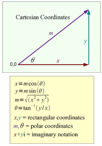 Figure 1: Coordinates
This page shows how Sage manages complex numbers in the analysis of electronic concepts like impedance. Since we're surrounded by electronics in all directions, I thought this would be a useful and educational example of what Sage can do.
Complex numbers aren't all that complex if they're pictured as two-dimensional vectors. Just think of a two-component Cartesian vector — its elements are at right angles to each other and its properties are easy to understand.
For a Cartesian vector, we might name the components x and y and think of them as the base and height of a right triangle (Figure 1). It's important to emphasize that the three notation systems in Figure 1 are equivalent and interchangeable — it's a matter of deciding which notation is appropriate to a particular problem.
In this article we'll be analyzing electronic RLC (resistor/inductor/capacitor) circuits, which possess a property called "impedance". Analyzing impedance naturally calls for complex numbers, because the currents flowing through an RLC circuit behave differently in each of the three components:
- For the resistor, voltage and current are synchronized in time, which means the resistor dissipates power (voltage times current) as heat.
- For the inductor, measured current represents the time integral of voltage (current lags voltage by 90°).
- Because an inductor's voltage and current are out of phase by 90°, an ideal inductor doesn't dissipate any power but stores energy as a magnetic field.
- For the capacitor, measured voltage represents the time integral of current (voltage lags current by 90°).
- Because a capacitor's voltage and current are out of phase by 90°, an ideal capacitor doesn't dissipate any power but stores energy as an electrical field.
For an RLC circuit and depending on the connection details, the circuit is appropriately described using equations involving complex numbers. Such a circuit is normally analyzed with respect to time-varying applied voltages — a typical example would be an RLC circuit driven by a signal generator.
Before we begin our topic, let's look at how Sage manages complex numbers. A mathematician would create a complex number like this:
z = x+yiWhere i2 = -1. Without providing all the details, this means that y is orthogonal (at right angles) to x. That in turn means we can treat x and y as a Cartesian vector (Figure 1) and derive some useful values.
Let's take the next steps in Sage. But first, as with my other articles in this series, let's put this initialization cell in a Sage worksheet (copy the content from this page or click here to download the complete Sage worksheet):
#auto
reset()
# special equation rendering
def render(x,name = "temp.png",size = "normal"):
    if(type(x) != type("")): x = latex(x)
    latex.eval("\\" + size + " $" + x + "$",{},"",name)
var('r_l r_c X_l X_c f a b c x y z zl zc r l c L C omega')
radians = pi/180.0
degrees = 180.0/pi

# define arg(x) in degrees
def argd(x):
    return N(arg(x) * degrees)

# complex plot function
def plt(q,a,b,typ = abs,col = 'blue'):
     return plot(lambda x: float(typ(q(x))),(x,a,b),rgbcolor=col)

omega = 2*pi*f

# series rlc circuit definition
zs(r,l,c,f) = r + (i*omega*l) - i/(omega*c)

# parallel rlc circuit definition
# from http://hyperphysics.phy-astr.gsu.edu/Hbase/electric/rlcpar.html#c2
zp(r_l,r_c,l,c,f) = ((r_l + i*omega*l)*(r_c - i/(omega*c))) / ((r_l+r_c)+i*(omega*l-1/(omega*c)))
Now we can move on to our example:
var('x y')
f(x,y) = x+y*i
Function f(x,y) constructs a complex number from the arguments x and y.
z = f(3,4) abs(z)5The Sage function "abs(x)" produces the "absolute value" of a number, which means different things depending on context. For a scalar (a one-component number, not a vector), it will do this:render(abs(x),"equ_abs_x.png","Large")Meaning abs(x) will produce an unsigned version of x. But for a complex number: abs(3+4*i)5
In this case, "abs(x)" produces the magnitude of the provided complex argument (or the hypotenuse of a right triangle with x and y as base and height, see Figure 1). It turns out that (3,4,5) is the first Pythagorean triple, which means 32 + 42 = 52.
Another useful complex number function is "arg(x)", which provides the angle component of its complex argument in radians, equal to tan-1(y/x) (this is θ in Figure 1):arg(3+4*i)0.927295218002Or, expressed in degrees (using a custom function in the initialization cell above):argd(3+4*i)53.1301023541560Intuitively, since 4 > 3, the angle should be more than 45 degrees.
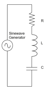 Figure 2: Series RLC Circuit
In electronics the term "reactance" refers to the behavior listed above for inductors and capacitors in which they store energy instead of dissipating it. The most important thing to understand about reactance is that voltage and current are orthogonal (at right angles), which explains why ideal inductors and capacitors don't dissipate any power (real-world reactors have some internal resistance, so they dissipate some power).
Remember that reactance is a dynamic property that depends primarily on the rate of change in current in the circuit containing the reactors. Consequently reactance is typically expressed with respect to frequency. Here are reactance equations for inductors and capacitors:
Capacitive reactance:(1)Inductive reactance: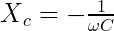 (2)Where:
 (3)
(3)
And f = frequency in Hertz. Above we mentioned impedance, which is the combination of resistance and reactance. Because reactances and resistances are orthogonal, we need to express this idea using complex numbers. Here is how we compute impedance (z) for a series RLC circuit:
(4)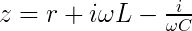
Note the presence of "i" (i2 = -1) in both the inductive and capacitive reactance subexpressions. This serves to keep the reactances at right angles to the resistance.
For such a circuit there is a resonant frequency where (in a series circuit as shown in Figure 2) the inductive and capacitive reactances become equal (and cancel out), as a result of which the current peaks and the phase angle between resistance and reactance becomes zero. We can plot this resonance point:
# series rlc circuit plot
# plotting range: a = start, b = end (Hertz)
a = 500
b = 2500
# r = .1 ohms, l = 100 microhenries, c = 100 microfarads
r = .1
l = 1e-4
c = 1e-4
q(f) = zs(r,l,c,f)
p1 = plt(1/q,a,b,abs,'#800000')
p2 = plt(q,a,b,arg,'#008000')
show(p1+p2,figsize=(4,3),axes_labels=('freq Hz','admittance $\mho$'))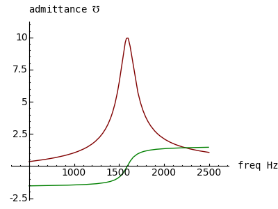
First, I am using a roundabout way to plot these results. This is required because of a bug in Sage 4.1.2 that prevents plotting complex numbers without some special precautions. I am calling a special function "plt()" that appears above in the worksheet initialization block.
In this graph the red trace represents admittance (with units of mhos or Siemens), because I decided to plot 1/q(f) rather than q(f) (with units of impedance), in order to produce a definite peak.
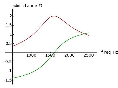
The green trace represents complex phase angle in radians, and according to the series RLC equation, at resonance it should become zero. In the graph this resonance appears to be located at about 1600 Hz. Here's the theoretical location of resonance (in Hertz):
(5)
Let's compute this value using Sage and our defined l and c values:
N(1/(2*pi*sqrt(l*c)))1591.54943091895Now let's see if our series RLC function "zs(r,l,c,f)" agrees with the theoretical prediction:
find_root(lambda f: float(arg(zs(r,l,c,f))),500,2500)1591.5494309189535For this example, the numerical root finder "find_root()" was able to find a zero using arg(x), which, as shown in the above graph, crosses zero at resonance. It should be pointed out that the "lambda f: float(arg())" construction is a temporary work-around for a bug in the current (4.1.2) version of Sage.
Another point about the above graph is that the red peak rises to about 10 mhos (units of admittance), which is consistent with our circuit's resistance value of .1 ohm and the fact that our "signal generator" is producing 1 volt.
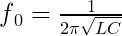
I ask my readers to think about the graph above. The current flowing in the circuit is proportional to the hypotenuse of a right triangle with the resistance representing the base, and both reactances representing the height. This means the steepness of the resonance curve should depend very much on the resistance. Let's find out by changing the resistance in the above code block to .01 Ω (r = 0.01):
We see a dramatic change in the steepness of the slopes, the height of the resonance peak and the abrupt phase change at resonance (green trace). Now let's change the resistance to 0.5 Ω:
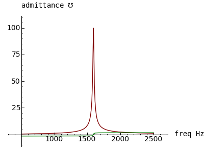
We see the opposite effect — a broadening of the resonance curve, a decrease in the amplitude of the resonance peak and a more gradual phase change near resonance. I want to emphasize to my readers that these results are perfectly consistent with physical measurement of actual circuits.
About these graphs, it would be nice to have two independent graph scales, one for the amplitude trace and another for the phase angle, so the green trace doesn't disappear when high admittance values are being plotted, but it seem Sage hasn't acquired that feature yet.
One more observation about circuits possessing impedance — it is almost never the case than one can determine the power being dissipated in the circuit by measuring voltage and current. The reason is that the voltage and current are nearly always out of phase with each other, and the actual power is roughly proportional to the voltage times the current, times the cosine of the phase angle between voltage and current.
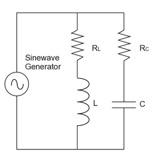 Figure 3: Parallel RLC Circuit
Let's move on to the parallel case (see Figure 3). This circuit is a bit more complex, having two resistances (rl and rc) to compute, and consistent with real-world parallel resonant circuits where both resistances must be taken into account. Many of the previously described reactance equations apply here, but computing impedance is somewhat more complex:
(6)
In this connection remember again that:
(7)And f = frequency in Hertz. Let's begin by plotting an example of this system:
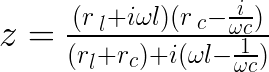
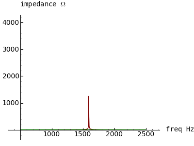
# parallel rlc circuit plot
# plotting range: a = start, b = end (Hertz)
a = 500
b = 2500
# r_l = .1 ohms, r_c = .1 ohms
# l = 100 microhenries, c = 100 microfarads
r_l = .1
r_c = .1
l = 1e-4
c = 1e-4
q(f) = zp(r_l,r_c,l,c,f)
p1 = plt(q,a,b,abs,'#800000')
p2 = plt(q,a,b,arg,'#008000')
show(p1+p2,figsize=(4,3),axes_labels=('freq Hz','impedance $\Omega$'))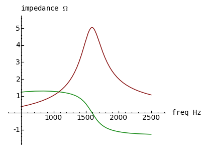
First, notice about this plot that the vertical axis is impedance, not admittance as with the series examples above. Notice that the phase versus frequency relationship is reversed compared to the series case, and that at resonance the impedance is 5Ω. The reason for the relatively low impedance is that currents within a parallel resonant circuit flow back and forth between the inductor and capacitor (the inductor stores energy as a magnetic field and the capacitor stores energy as an electrical field), but because of the circuit layout (Figure 3), this flow is resisted by both rl and rc. Try setting rl to 0Ω in the above Sage plotting code and see what happens:
The impedance is now 10Ω at resonance. Think about this — at the circuit's resonant frequency we have increased the circuit's overall impedance by decreasing one of the resistances. Remember that, in this idealized circuit, the resistors are the only devices able to dissipate power. Isn't it ironic that we can increase impedance by decreasing a resistance?
Again, the reason for this is that an ideal parallel RLC circuit with no resistances should dissipate no power and should therefore have infinite impedance at resonance (and zero impedance everywhere else). Let's test this idea — set both rl and rc to .0001Ω and plot the result:
Well, that's clearly not right, and I suspect it's because the plot routine isn't providing enough resolution near resonance. So let's narrow the plot range — in the plotting code listed above, set variable a to 1580 and b to 1600, for this result:
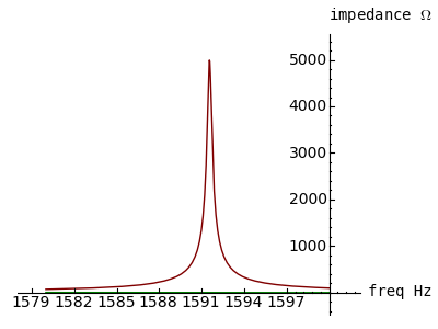
That's more like it. Remember this about parallel-resonant circuits — the impedance at resonance is determined by the distributed resistances in the circuit, and if they could be eliminated, the impedance at resonance would be infinite, but for an infinitely narrow bandwidth. Real-world circuits tend to have a finite bandwidth and a finite impedance, as shown by the first few graphs in this section.
A careful examination of Figure 3 above will reveal that, at f << f0 (f0 = resonant frequency), resistor rl should the the primary factor, and at f >> f0, resistor rc should be the primary factor. Let's find out — let's give rl and rc distinctive values and produce numerical results for f much less than, and much greater than, f0. Remember that the parallel circuit function "zp()" is defined as:
z = zp(rl,rc,l,c,f)Where:
- z = impedance, Ω
- rl = resistance on inductor leg, Ω
- rc = resistance on capacitor leg, Ω
- l = inductance, Henries
- c = capacitance, Farads
- f = frequency, Hertz
Result for rl = 7, rc = 13, f << f0:
N(abs(zp(7,13,1e-4,1e-4,1e-12)))7.00000000000000Result for rl = 7, rc = 13, f >> f0:
N(abs(zp(7,13,1e-4,1e-4,1e12)))13.0000000000000The reason for this result is that, at frequencies much less than f0, the capacitive reactance (Xc) becomes very high and the inductive reactance (Xl) becomes very low, which causes rl to predominate, but at frequencies much greater than f0, it's the opposite. It would be nice to see this result on a log scale ... hold on, I think I can do that using a text printout. For rl = 0.25 and rc = 0.75:
for n in range(0,7):
    print "f = 10^%d, z = %5.2f" % (n,N(abs(zp(.25,.75,1e-4,1e-4,10^n))))
f = 10^0, z = 0.25 f = 10^1, z = 0.25 f = 10^2, z = 0.26 f = 10^3, z = 0.86 f = 10^4, z = 0.78 f = 10^5, z = 0.75 f = 10^6, z = 0.75One can see the resonance peak even at this crude resolution. Hmm — maybe we can plot this relationship after all, even though we don't have an explicit log x scale:
# parallel rlc circuit log/linear plot
# plotting range: a = start, b = end, units f*10^n
a = 0
b = 7
r_l = .25
r_c = .75
l = 1e-4
c = 1e-4
q(n) = zp(r_l,r_c,l,c,10^n)
p1 = plt(q,a,b,abs,'#800000')
show(p1,figsize=(4,3),axes_labels=('$f = 10^n Hz$','impedance $\Omega$'),ymin=0)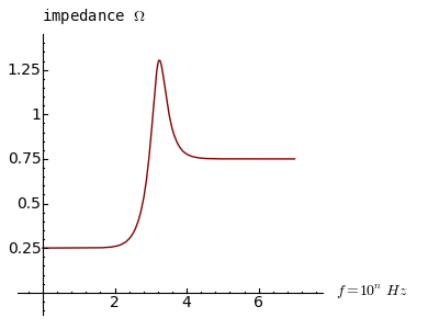
This plot clearly shows how rl and rc predominate in domains far from resonance. I chose resistances of 0.25Ω and 0.75Ω to get a positive peak at resonance, but if the resistances are > 1Ω, we get a very different result. Set rl = 1.25, rc = 1.75 in the above code block for this plot:
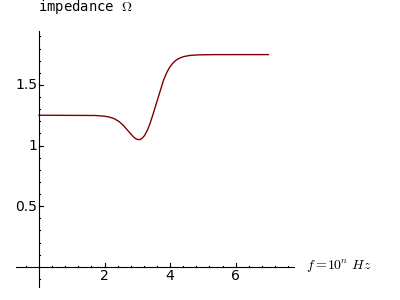
Think about that result — the impedance at resonance is less than the resistance value in either leg. Now make one more plot — set both rl and rc to 1Ω. I won't reveal the result — it defies expectation, but a clue can be seen in the above two plots.
This kind of virtual circuit modeling is a very fruitful way to learn about electronic circuits in a short time, especially when compared to building and testing actual circuits. It's also a great deal less expensive. I must say, even though I've designed circuits for years including some aboard the NASA Space Shuttle, I didn't know about the outcome for two resistances of 1Ω in a parallel-resonant circuit. Even though I never realized it before, I can picture the reason (it has to do with internal versus external currents). And if I hadn't built a model, I would never have known about it.
I've been using computer algebra systems for years, and what impresses me most about Sage is the speed with which one acquires useful results, as well as the fact that one can easily export a decent graphic of an equation or a plot (for me personally, that's a revelation).
Those familiar with the conventions of electronic calculation may object to my having used i as the complex operator (i2 = -1) — in electrical work, i normally stands for current and this conflicts with its other meaning. For those who prefer to use j instead of i, Sage makes this very simple:
j=i i=0 j^2-1I want to close with a discussion of the symbolic representation for admittance, the reciprocal of impedance, expressed in the unit "mho" (that's ohm spelled backwards, if you missed it) or "Siemens" in SI units. First, there isn't a defined HMTL entity for this symbol, so when writing HTML one must use either a graphic image or an explicit Unicode value: ℧ = ℧ (this might fail on some browsers or systems without Unicode font support).
When presented with "\mho", TeX-capable systems like Sage produce this:
"\mho" ->In contrast with the symbol for "ohm" (uppercase Greek Omega): "\Omega" ->
But isn't it obvious that:
Just as:

I expect eventual mass confusion.
"Exploring Mathematics with Sage" by Paul Lutus is licensed under a
Creative Commons Attribution-Noncommercial-Share Alike 3.0 United States License.
| Home | | Mathematics | | * Sage | | | | Share This Page |