Share This Page
| Home | | Mathematics | | Signal Processing | | | | Share This Page |
A practicum on Fourier analysis and signal processing
— P. Lutus — Message Page —
Copyright © 2008, P. Lutus
(double-click any word to see its definition)
Before describing the Fourier Transform, we need to describe some mathematical notation conventions. The data processing methods described in this article depend on the use of "complex numbers," that is, numbers having two orthogonal components (components separated by 90°). One way of interpreting these numbers is as having "real" and "imaginary" components, but this convention is only one way to describe what are in fact two-dimensional Cartesian vectors, numbers that have both magnitude and direction (contrast this with a scalar, a number with only a magnitude).
The "complex number" convention has certain computational advantages, and for this convention, a number pair (x,y) is written like this:
x + iy
Where i = the square root of -1. As it turns out, multiplying a number by i has the effect of rotating it through 90 degrees, so this operation provides the expected 90° relation between the components.
Regardless of whether one thinks of these number pairs as "real" and "imaginary", or "x" and "y" points on a Cartesian plane, it is important to understand that the various notational conventions are interchangeable — they are equivalent descriptions of a two-dimensional vector.
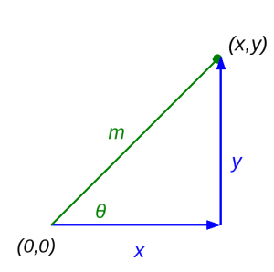
There is even a third way to describe a vector — the "polar notation". Consider this diagram:
In this diagram, we have:
Rectangular to Polar (x,y) -> (m,θ):
Polar to Rectangular (m,θ) -> (x,y):
In signal processing work, complex numbers and vectors are ubiquitous, so it is a good idea to become comfortable with their various representations. We've just described three vector representations, all equivalent, with different best uses — complex (x+iy), rectangular (x,y) and polar (m,θ).
It is also useful to visualize vectors in particular ways — for example, a vector that represents a time-varying sinewave can be thought of as the spinning hand of a clock, with a full sinewave cycle represented by a complete rotation of the hand. Look at the vector diagram above and imagine the green m "magnitude" line rotating around the (0,0) point, and think about the resulting x and y values. A bit of thought and visualization like this can help one imagine the result of multiplying two vectors together, an operation at the heart of the Fourier Transform.
In signal processing, the primary operation is conversion between time and frequency domains. The Fourier Transform (FT) converts a time-varying function into the frequency domain, and the Inverse Fourier Transform (IFT) converts a frequency-domain function into the time domain. Not unlike derivation and integration in Calculus, the FT and IFT are reciprocal operations — all things being equal, the IFT of an FT should produce the original function or data set.
The Fourier Transform (conversion from the time domain to the frequency domain) is defined as:
While the Inverse Fourier Transform (frequency to time domain) is defined as:
Where:
As it turns out and fortunately, the following relation holds (Euler's Formula):
And therefore:
It is only because of the relation expressed in Euler's Formula that we can write practical tools based on the Fourier Transform.
Because we would like to apply these ideas to a signal source rather than a mathematical function, we will now examine the Discrete Fourier Transform (DFT), a method that can be applied to a collection of real-world data points. The Discrete Fourier Transform (DFT) (time domain to frequency domain) is defined as:
While the Inverse Discrete Fourier transform (IDFT) (frequency domain to time domain) is defined as:
Where:
It may not be clear to the nontechnical reader, but the DFT and IDFT expressions above require nested loops, one for n and one for k, as a result the solution time increases as O(N2), consequently this method is not practical for most real-world data sets. The value of the DFT lies, not in processing data, but in clarifying technical issues.
| Home | | Mathematics | | Signal Processing | | | | Share This Page |